PS Flash Solver Numerical Instability
2026-11-13
Problem
When calculating a single-phase thermodynamic state, a pressure-entropy (PS) flash solver can become unstable as the state approaches the critical point. This note formulates the two-variable Newton method, derives the required thermodynamic derivatives and the discusses the conditioning of the Jacobian.
PS Flash Solver
Given pressure ($P_s$) and entropy ($s_s$), the PS flash solver will find temperature $T$ and density $\rho$ satisfying the following two equations:
\[P(T, \rho) = P_s\] \[s(T, \rho) = s_s\]Define the residual functions $f_1$ and $f_2$,
\[f_1(T, \rho)=P(T, \rho) - P_s\] \[f_2(T, \rho)=s(T, \rho) - s_s\]The problem is to find roots of the following equation system,
\[\begin{cases} f_1(T, \rho) = 0.0 \\ f_2(T, \rho) = 0.0 \end{cases}\]The Newton iterative algorithm is shown,
\[J^{(n)} \begin{bmatrix} \triangle T \\ \triangle \rho \end{bmatrix} = - \begin{bmatrix} f_1^{n} \\ f_2^{n}\end{bmatrix}\]where
\[J = \begin{bmatrix} \frac{\partial P}{ \partial T} & \frac{\partial P}{ \partial \rho} \\ \frac{\partial s}{ \partial T} & \frac{\partial s}{ \partial \rho} \end{bmatrix}\]and,
\[T^{(n+1)}=T^{(n)} + \triangle T\] \[\rho^{(n+1)}=\rho^{(n)} + \triangle \rho\]Numerical Stability
The numerical stability depends on Jacobian matrix condition. In the next sections, we will review. The determinate of the Jacobian matrix is,
\[det(J)= \left( \frac{\partial P}{ \partial T} \right)_\rho \left( \frac{\partial s}{ \partial \rho} \right)_T - \left( \frac{\partial P}{ \partial \rho} \right)_T \left( \frac{\partial s}{ \partial T} \right)_\rho\]Thermodynamic Derivatives
Step 1
From the thermal dynamic identities,
\[Tds = du + Pdv\]Here $v = 1/ \rho$.
At constant density, $Pdv=0$. Thus,
\[Tds = du\]Re-arrange,
\[\left( \frac{\partial s}{\partial T} \right)_\rho = \frac{1}{T} \left( \frac{\partial u}{\partial T} \right)_v\]By definition of heat capacity at constant-volume,
\[du = c_v dT\]This gives,
\[c_v= \left( \frac{\partial u}{\partial T} \right)_v\]and thus,
\[\left( \frac{\partial s}{\partial T} \right)_\rho = \frac{c_v}{T}\]Note: constant $\rho$ is equivalent of constant $v$ as $v = 1/\rho$.
Step 2
From Helmholtz thermodynamics identity,
\[da = -sdT -Pdv\]where $a$ is the specific Helmholtz energy.
Because $v=1/\rho$,
\[dv = -\frac{1}{\rho^2}d\rho\]We then have,
\[da = -sdT + \frac{P}{\rho^2}d\rho\]With Maxwell relationship, we get,
\[\left( \frac{\partial (-s)}{\partial \rho} \right)_T= \left( \frac{\partial {(P/\rho^2)}}{\partial T} \right)_\rho\]re-arrange the equation,
\[\left( \frac{\partial s}{\partial \rho} \right)_T= -\frac{1}{\rho^2}\left( \frac{\partial {P}}{\partial T} \right)_\rho\]Step 3
The total differential of entropy is,
\[ds = \left( \frac{\partial s}{\partial T} \right)_\rho dT + \left( \frac{\partial s}{\partial \rho} \right)_T d\rho\]With results of step 1 and 2,
\[ds = \frac{c_v}{T} dT -\frac{1}{\rho^2}\left( \frac{\partial {P}}{\partial T} \right)_\rho d\rho\]Divide both sides with $dT$ under constant pressure,
\[\left( \frac{\partial {s}}{\partial T} \right)_P = \frac{c_v}{T} -\frac{1}{\rho^2}\left( \frac{\partial {P}}{\partial T} \right)_\rho \left( \frac{\partial \rho}{\partial T} \right)_P\]On the other hand, at constant pressure,
\[dP = \left( \frac{\partial P}{\partial T} \right) _\rho dT + \left( \frac{\partial P}{\partial \rho} \right) _Td\rho =0\]Rearranging,
\[\left( \frac{\partial \rho }{\partial T} \right) _P= - \frac { \left( \frac{\partial P}{\partial T} \right) _\rho} { \left( \frac{\partial P}{\partial \rho} \right) _T}\]Therefore,
\[\left( \frac{\partial {s}}{\partial T} \right)_P = \frac{c_v}{T} +\frac{1}{\rho^2}\left( \frac{\partial {P}}{\partial T} \right)_\rho \frac { \left( \frac{\partial P}{\partial T} \right) _\rho} { \left( \frac{\partial P}{\partial \rho} \right) _T}\]By definition,
\[c_p = \left( \frac{\partial q}{\partial T} \right) _P=T \left( \frac{\partial s}{\partial T} \right) _P\]Then,
\[\frac{c_p}{T} = \frac{c_v}{T} +\frac{1}{\rho^2}\left( \frac{\partial {P}}{\partial T} \right)_\rho \frac { \left( \frac{\partial P}{\partial T} \right) _\rho} { \left( \frac{\partial P}{\partial \rho} \right) _T}\]This gives,
\[c_p - c_v = \frac{T}{\rho^2} \frac { \left( \frac{\partial P}{\partial T} \right) _\rho^2} { \left( \frac{\partial P}{\partial \rho} \right) _T}\]Step 4
The determinate of the Jacobianmatrix is,
\[det(J)= \left( \frac{\partial P}{ \partial T} \right)_\rho \left( \frac{\partial s}{ \partial \rho} \right)_T - \left( \frac{\partial P}{ \partial \rho} \right)_T \left( \frac{\partial s}{ \partial T} \right)_\rho\]Substitudes the results from step 1 to step 3, we have,
\[\begin{aligned} det(J) &= - \left( \frac{\partial P}{ \partial T} \right)_\rho \frac{1}{\rho^2}\left( \frac{\partial {P}}{\partial T} \right)_\rho - \left( \frac{\partial P}{ \partial \rho} \right)_T \frac{c_v}{T} \\[1em] &= - \frac{c_p -c_v}{T}\left( \frac{\partial P}{\partial \rho} \right) _T - \frac{c_v}{T} \left( \frac{\partial P}{ \partial \rho} \right)_T \\[1em] &= -\frac{c_p}{T}\left( \frac{\partial P}{\partial \rho} \right) _T \end{aligned}\]Step 5
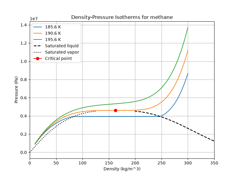
For a pure fluid at the critical point, $\left( \frac{\partial P}{\partial \rho} \right) _T \rightarrow 0 $ (see Figure 1).
From step 3 (also the formula below), when $\left( \frac{\partial P}{\partial \rho} \right) _T \rightarrow 0 $, $c_p \rightarrow \infty $.
\[c_p - c_v = \frac{T}{\rho^2} \frac { \left( \frac{\partial P}{\partial T} \right) _\rho^2} { \left( \frac{\partial P}{\partial \rho} \right) _T}\]Or , we can write,
\[\begin{aligned} det(J) &= -\frac{c_p}{T}\left( \frac{\partial P}{\partial \rho} \right) _T \\ &=- \frac{c_v}{T}\left( \frac{\partial P}{\partial \rho} \right) _T - \frac{1}{\rho^2}\left( \frac{\partial P}{\partial T} \right) _\rho^2 \\ &\rightarrow - \frac{1}{\rho^2}\left( \frac{\partial P}{\partial T} \right) _\rho^2 \end{aligned}\]Though $ \left( \frac{\partial P}{\partial T} \right) _\rho$ can approach a limit value, the calculation involves division by zero and infinite value. This can cause numerical instability.