Pipe Flow Modelling Accuracy
2026-10-16
Pipe Flow
Problem:
Air (20 degC and 1 atm) flow through a pipe (length: 1m and diameter 0.1m) with an average flow velocity 0.01m/s.
Question:
How accurate of the pressure drop the model predition is?
Assumptions:
- The flow is fully developed.
- The pipe cross section is circular.
Theoretical Pressure Drop
For air at 20 degC and 1 atm, the kinematic viscosity can be found from a reference $1.51\times 10^{-5}$ $m^2/s$ and density 1.204 $kg/m^3$.
The Reynolds number is then calculated,
\[Re_D = \frac{D \cdot U}{\nu}=66.2\]The Reynolds number is less that the critical Reynolds number 2300. Thus the flow is laminar.
The pressure drop is estimated with Darcy-Weisbach equation,
\[\frac{\triangle p}{L}=f_D \cdot \frac{\rho}{2} \cdot \frac{U^2}{D}\]where, the Darcy friction factor, for laminar flow, is,
\[f_D = \frac{64}{Re}=0.9664\]This gives theoretical pressure drop: $5.82\times 10^{-4}$ Pa.
CFD Model
A 2D axi-symmetric model is built. The solver is incompressive laminar flow simpleFoam. The wall boundary condition is noSlip. The inlet boundary condition uses the following parabolic velocity profile with type codedFixedValue. This is convenient as the flow is fully developed and laminar.
Mesh is uniform. Simulations were made with 3 cell sizes (fine 3.8mm, medium 4.9mm and coarse 6.4mm). The refinement ratio is kept 1.3. Note the cell size is representive cell size which is estimated from the total domain volume and cell count.
The pressure drop results are listed in the table below.
| Mesh Cell Size (m) | Pressure Drop (Pa) |
|---|---|
| 0.0038 | 5.81E-4 |
| 0.0049 | 5.78E-4 |
| 0.0064 | 5.73E-4 |
The plot below displays the result and the curve fit with 2nd order polynomial. Note in the plot, extra computation results of smaller cell size are given.
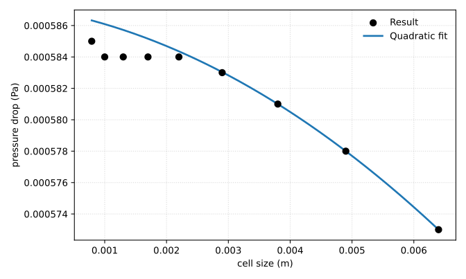
As can be seen, when the cell size reaches 2.2mm, the results are independent to the mesh size except the last point with cell size 0.79mm. The last point may experience convergence issue when the cell size is very small.
Model Accuracy
From the above CFD results, we can estimate the model accuracy.
Cell Refinement Ratio:
\[r=r_{21}=r_{32}=1.3\]Solutions:
\[\phi_1 = 5.81 \times 10^{-4}\] \[\phi_2 = 5.78 \times 10^{-4}\] \[\phi_3 = 5.73 \times 10^{-4}\]Solution differences:
\[\epsilon_{21}=\phi_2-\phi_1= -2.8641 \times 10^{-6}\] \[\epsilon_{32}=\phi_3-\phi_2= -5.0626 \times 10^{-6}\]Order of Accuracy:
\[p=\frac{ln|\epsilon_{32}/\epsilon_{21}|}{ln(r)}=2.1\]Richardson Extrapolation:
\[\phi=\phi_1+\frac{\phi_1-\phi_2}{r^p-1}=5.85\times 10^{-4}\]Comparing to theoretical value $5.82\times 10^{-4}$, the error is 0.56%, which seems a pretty good approximation.
Convergence Ratio (R):
\[R=\frac{\epsilon_{21}}{\epsilon_{32}}=0.56\]The convergence ratio is between 0 and 1. Thus, it is monotonic convergence.
Estimated Error:
Without using theoretical value, the estimated error is,
\[E_{21}=\frac{\phi_1-\phi_2}{\phi_1(r^p-1)}=0.64 \%\] \[E_{32}=\frac{\phi_2-\phi_3}{\phi_2(r^p-1)}=1.14 \%\]Note the error of $\phi_1$ is very close to that of Richardson extrapolation result.
Grid Convergence Index (GCI):
\[GCI_{21}=F_s \cdot E_{21} = 0.80 \%\] \[GCI_{32}=F_s \cdot E_{32} = 1.43 \%\]$CGI_{21}$ is less than 1 and can be generally assumed to be accurate and mesh independent.
Asymptotic Ratio (AR):
\[AR =\frac{GCI_{32}}{r^p\cdot GCI_{21}}=1.00\]As AR is close to 1.0, the grid refinement is within the asymototic range.
CFD Result Error:
Now we come to estimate the CFD predicted pressure drop error.
\[\triangle p= \phi_1 \pm (\phi_1 \cdot GCI_{21}) = 5.81 \times 10^{-4} \pm 0.05 \times 10^{-4} Pa\]The range, when it is in the above plot, is quite large, though the accuracy is acceptablly below 1%.
Notes
Without using parabolic velocity profile, the pipe flow entrance effect should be considered. In case, one use uniform velocity inlet boundary condition, the result would be still fine but not comparable to the theoretical calculated result assuming fully developed laminar flow.
For turbulent flow, it would be difficult to set up a fully developed flow inlet boundary condition. In addition, because we will use law of wall bondary condition (standard k-epsilon model or SST k-omega model), the mesh refinement should be carried out carefully; one would like to keep $y^+$ in a range of 30 to 300. When $y^+$ is less than 30, CFD results would yield significant error.